A flow to Test Your Hypothesis in Python

Overview#

All the practitioners of data science always hit one giant thing to do with data and you know it well its EDA -Exploratory Data Analysis. This word EDA¹ was coined by Tukey himself in his seminal book published in 1983. But do you think that before that EDA doesn’t existed ?

Well glad you thought. Before that all were doing what is called as Hypothesis Testing. Yes, before this the race was majorly to fit the data and make most unbiased and robust estimate. But remember one thing when you talk about Hypothesis Testing it was always and majorly would be related to RCTs (Randomized Controlled Trials) a.k.a Randomized Clinical Trials and is Gold Standard of data.

More on RCTs and ODs#

Now let me now not hijack the discussion to what is RCTs and Observational Data (ODs) as it is more of Philosophical Reasoning rather than other quality of data, but essentially what we are trying to find is that can we by, using stats, identify interesting patterns in data.

The only thing happens wit RCT data is that we tend to believe these interesting patterns coincide with some sort of ‘Cause-Effect’ kind of relationship. But essentially due to bia nature of ODs, we certainly cant conclude this. And hence, can only find interesting patterns.

Lets move on. The big question is, for whatever reason you are doing HT , you are doing it for finding something intreating. And that something interesting is usually found by using Post-Hoc Tests. Now there are variety of Post-Hocs available but what is more know and hence easily found to be implemented in Tukey’s HSD.

So lets directly jump to how to follow this procedure. We’ll be using bioinfokit for this, as it is much simpler wrapper around whats implemented in statsmodels.

What are the results#

Pheww… Thats too much code right. But that would save a lot of your time in real life. So in real life you would write code as 3 steps below:

# import libraries
import pandas as pd

# Getting car data from UCI
df = pd.read_csv('https://archive.ics.uci.edu/ml/machine-learning-databases/auto-mpg/auto-mpg.data',
				 sep='\s+',header=None,
				 names=['mpg','cylinders','displacement','horsepower','weight',
				 'acceleration','model_year','origin','car_name'])
df.head()

# Syntax to do anove with validating the assumption, doing test and a post-hoc
results = do_anova_test(df=df, res_var='mpg',xfac_var='cylinders', 
                        anova_model='mpg ~ C(cylinders)+C(origin)+C(cylinders):C(origin)',
                        ss_typ=3, result_full=True)

Results form the do_anova_test

Levens Test Result:
                 Parameter    Value
0      Test statistics (W)  14.5856
1  Degrees of freedom (Df)   4.0000
2                  p value   0.0000

Bartletts Test Result:
                 Parameter    Value
0      Test statistics (T)  61.2143
1  Degrees of freedom (Df)   4.0000
2                  p value   0.0000

ANOVA\ANCOVA Test Result:
                           df     sum_sq    mean_sq         F  PR(>F)      n2
Intercept                 1.0  6195.1701  6195.1701  296.3452  0.0000  0.2727
C(cylinders)              4.0  7574.5864  1893.6466   90.5824  0.0000  0.3334
C(origin)                 2.0   241.0703   120.5351    5.7658  0.0034  0.0106
C(cylinders):C(origin)    8.0   577.4821    72.1853    3.4530  0.0046  0.0254
Residual                389.0  8132.1404    20.9052       NaN     NaN     NaN

Tukey HSD Result:
   group1  group2     Diff    Lower    Upper  q-value  p-value
0       8       4  14.3237  12.8090  15.8383  36.6527   0.0010
1       8       6   5.0226   3.1804   6.8648  10.5671   0.0010
2       8       3   5.5869  -0.7990  11.9728   3.3909   0.1183
3       8       5  12.4036   5.0643  19.7428   6.5503   0.0010
4       4       6   9.3011   7.6765  10.9256  22.1910   0.0010
5       4       3   8.7368   2.4102  15.0633   5.3524   0.0017
6       4       5   1.9201  -5.3676   9.2078   1.0212   0.9000
7       6       3   0.5643  -5.8486   6.9772   0.3410   0.9000
8       6       5   7.3810   0.0182  14.7437   3.8854   0.0491
9       3       5   6.8167  -2.7539  16.3873   2.7606   0.2919

Nice!!!

And plotting is even easier

# Numbers are clumsy for most. Making more interpretable plot on above results.
plot_hsd(results.tukeyhsd.sort_values('Diff'), title="Tukey HSD resutls Anova of MPG ~ Cylinder")

Results form the plot_hsd

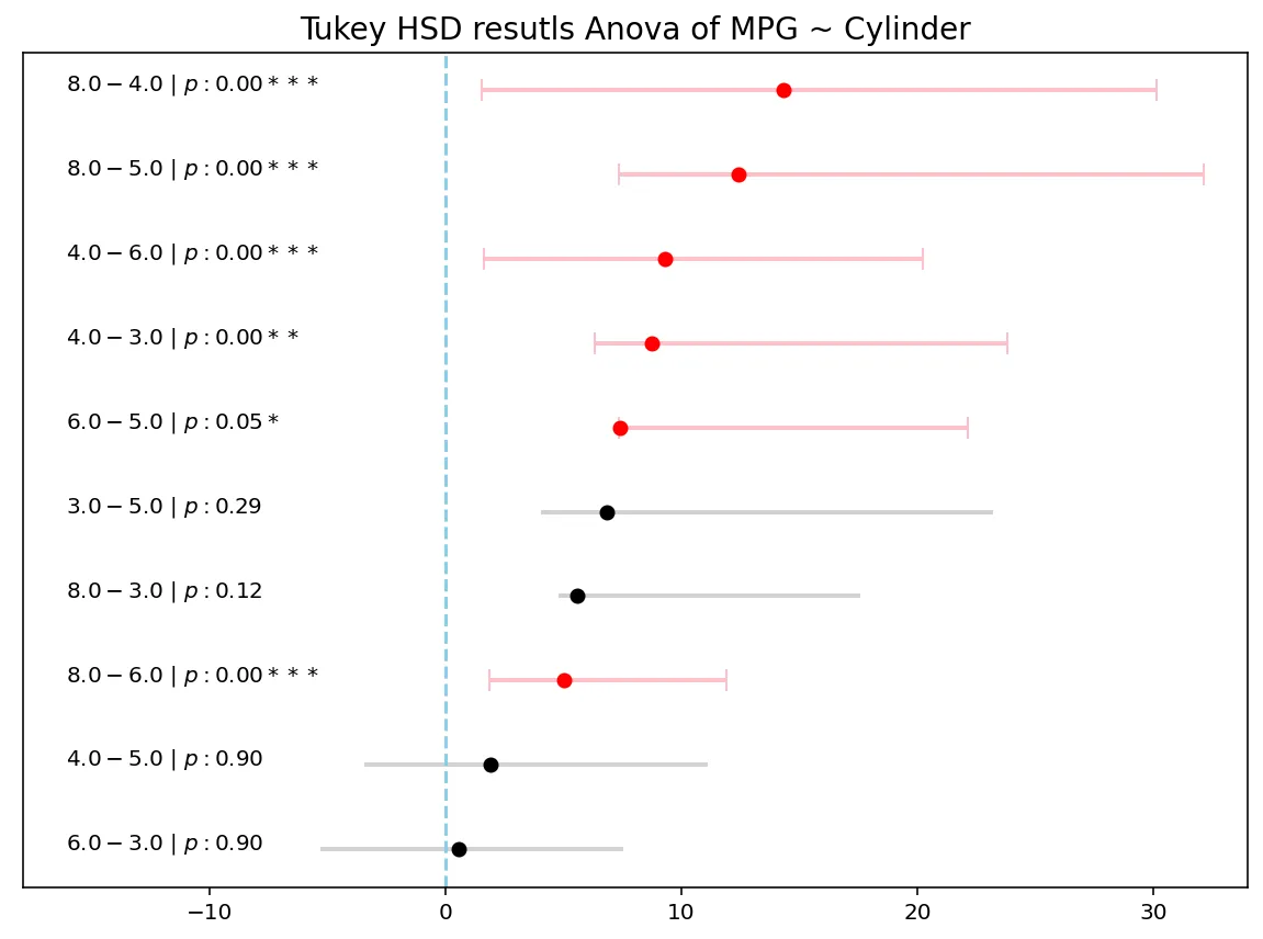
Plots look good with ‘p-values’.

Conclusion#

Now since we applied the above to a Non RCT we cannot conclude that Difference in mpg based on cylinder is huge specially as number of cylinders goes up. But this statement might not be as explicit as might be appearing from plot. Unless you have a strong believe that the data follows with rules and assumptions of RCTs, we should be only seeking interesting as in associated results and not cause-effect results.

Give me “The Code”#

Performing Anova#

from bioinfokit import analys

import numpy as np
from scipy import stats

class KeyResults:
    """
    A basic class to hold all the results
    """
    
    def __init__(self,result_full):
        self.keys = []
        self.result_full = result_full
    
    def add_result(self,name,result):
        if name == 'tukeyhsd':
            self.keys.append(name)
            setattr(self, name, result)
        elif self.result_full:
            self.keys.append(name)
            setattr(self, name, result)

# Anova test code
def do_anova_test(df, res_var, xfac_var, anova_model,ss_typ=3,
				  effectsize='n2',result_full=False,add_res=False):
    """
    Do all sequential anova tests
    
    Step 1) Leven's/ bartellet test for checking weather variance is homogenous or not
    Step 2) Main ANOVA/ANCOVA test
    Step 3) Tukey's HSD for individual combinations
    
    :param df: Pandas DataFrame holding all the columns
    :param res_var: Variable for which we are checking ANOVA
    :param xfac_var: Grouping Variables for which we want to do the comparisons
    :param anova_model: SM formula for the model. This is life savour to make all things work
    :param result_full: To provide all the results of intermediate steps
    
    """

    results = KeyResults(result_full)
    
    # initialize stat method
    res = analys.stat()
    
    # doing levens test
    res.levene(df=df, res_var=res_var,xfac_var=xfac_var)
    print('\nLeven\'s Test Result:')
    print(res.levene_summary)
    results.add_result('levene',res.levene_summary)

    # doing bartlett test
    res.bartlett(df=df, res_var=res_var,xfac_var=xfac_var)
    print('\nBartlett\'s Test Result:')
    print(res.bartlett_summary)
    results.add_result('bartlett',res.bartlett_summary)
    
    # doing anova / ancova
    res.anova_stat(df=df, res_var=res_var, anova_model=anova_model,ss_typ=ss_typ)
    aov_res = res.anova_summary
    
    # Add effect sizes
    if effectsize == "n2":
        all_effsize = (aov_res['sum_sq'] / aov_res['sum_sq'].sum()).to_numpy()
        all_effsize[-1] = np.nan
    else:
        ss_resid = aov_res['sum_sq'].iloc[-1]
        all_effsize = aov_res['sum_sq'].apply(lambda x: x / (x + ss_resid)).to_numpy()
        all_effsize[-1] = np.nan
    aov_res[effectsize] = all_effsize
    #aov_res['bw_'] = res.anova_model_out.params.iloc[-1]
    aov_res = aov_res.round(4)
    
    # printing results
    print('\nANOVA\ANCOVA Test Result:')
    print(aov_res)
    results.add_result('anova',res.anova_summary.round(4))
    results.add_result('anova_model',res.anova_model_out)
    
    # doing tukey's hsd top compare the groups
    res.tukey_hsd(df=df, res_var=res_var,xfac_var=xfac_var, anova_model=anova_model,ss_typ=ss_typ)
    print('\nTukey HSD Result:')
    print(res.tukey_summary.round(4))
    results.add_result('tukeyhsd',res.tukey_summary.round(4))
    
    # add all result componets again if needed 
    if add_res:
        results.add_result('allresult',res)
    
    return results

Plotting Results#

import seaborn as sns
import matplotlib.pyplot as plt

plt.style.use('seaborn-bright')

def plot_hsd(hsdres,p_cutoff=0.05,title=None,ax=None,figsize=(10,7)):
     """
     Do plotting of tukeyhsd results
    
  
    :param hsdres: 'tukeyhsd' result form the do_anova_test function
    :param p_cutoff: Cutoff at which we get say a combination is significant
    :param title: Title of the plot
    :param ax: Define or get the matplotlib axes
    :param figsize: Mention Figure size to draw
    
    """

    if ax is None:
        fig,axp = plt.subplots(figsize=figsize)
    else:
        axp = ax
    
    # helper func
    p_ind = lambda x : '' if x > 0.1 else ('+' if x > 0.05 else ('*' if x > 0.01 else ('**' if x >0.001 else '***')))
    label_gen  = lambda x: f"${x[0]} - {x[1]}\ |\ p:{x[2]:0.2f}{p_ind(x[2]):5s}$"
    
    #setting values
    mask = hsdres['p-value'] <= p_cutoff
    yticklabs = hsdres[['group1','group2','p-value']].apply(label_gen,axis=1).values
    ys = np.arange(len(hsdres))
    
    # adding plot to axes
    axp.errorbar(hsdres[~mask]['Diff'],ys[~mask],xerr=np.abs(hsdres[~mask][['Lower',"Upper"]]).values.T,
                fmt='o', color='black', ecolor='lightgray', elinewidth=2, capsize=0)
    axp.errorbar(hsdres[mask]['Diff'],ys[mask],xerr=np.abs(hsdres[mask][['Lower',"Upper"]]).values.T,
                fmt='o', color='red', ecolor='pink', elinewidth=2, capsize=5)
    axp.axvline(x=0,linestyle='--',c='skyblue')
    axp.set_yticks([])
    (l,u) = axp.get_xlim()
    axp.set_xlim(l+1.5*l,u)
    (l,u) = axp.get_xlim()
    for idx,labs in enumerate(yticklabs):
        axp.text(l-0.1*l,ys[idx],labs)
    axp.set_yticklabels([])
    
    # finally doing what is needed
    if ax is None:
        plt.title('' if title is None else title,fontsize=14)
        plt.show()
    else:
        return axp

Hope this give you kickstart to find you intresting patterns. Happy Learning!

Footnotes#

1. Emerson, J. D., & Hoaglin, D. C. (1983). Stem-and-leaf displays. In D. C. Hoaglin, F. Mosteller, & J. W. Tukey (Eds.) Understanding Robust and Exploratory Data Analysis, pp. 7–32. New York: Wiley. Book is here. ↩