Predictive Maintenance: How AI Agents Draft Work Orders
Predictive maintenance alerts on manufacturing telemetry need context. An AI agent can inspect the readings and draft a work order for a technician to review.
Imagine an alarm flashing red on the telemetry console of an automated CNC machining cell:
WARNING: SPINDLE ASSEMBLY 04 - ANOMALY SCORE 0.87 (HIGH RISK)
The night technician checks the housing, oil pressure and motor. It sounds normal.
“Sensor’s crying wolf again,” he muttered. He hit ACKNOWLEDGE, silenced the buzzer, and went back to his logbook.
Later, a cutting tool fails under a high-torque pass and the cell stops.
The bill includes ruined stock, a replacement part and unscheduled shutdown.
In this illustrative incident, the data science lead points to the dashboard: “The detector gave a warning. Operations ignored the signal.”
The technician counters: “Most alerts are harmless vibration spikes when the air conditioning turns on. If I shut the line down every time your screen turns red, we’d never ship a part.”
The decision is which alert deserves a check, and what a technician should do next.
Connecting an LLM agent to an anomaly score can carry the same problem into the work-order queue. A high score alone does not justify dispatch or a change to the machine.
To build an agent that operations can trust, give it an auditable risk estimate and an approval path. A model tree is one way to expose the rule behind an estimate.
Why Do Predictive Maintenance Alerts Cause Alarm Fatigue?
A threshold alert can mistake a harmless change for a fault; a temperature differential gives a technician more context to investigate.
Think about the smoke detector in your kitchen.
It has one job: sound an 85-decibel screech when particulate density crosses a fixed threshold. It does not know whether the air contains smoke from an electrical fire inside the wall or steam from boiling pasta. It has no gradient, no context, and no explanation.
If you connected that smoke detector to an automated dispatch system, the fire brigade would be parked outside your house every Sunday morning when you make toast.
Now consider an industrial thermal gradient monitor.
It does not simply scream when temperature rises. It tracks the rate of change across two probes:
- Probe A measures ambient air temperature.
- Probe B measures the motor bearing housing.
If both probes rise together during a hot afternoon, the differential remains flat. That alone does not prove the machine is healthy. But if the housing temperature climbs while the ambient air stays cool, the difference gives the technician a reason to investigate local heating.
A smoke detector produces alarm fatigue. A thermal gradient meter produces diagnostic telemetry.
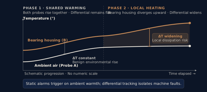 The difference between two signals is more useful than either alarm alone.
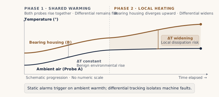 The difference between two signals is more useful than either alarm alone.
Scroll sideways to explore the full diagram.
TRADITIONAL PREDICTIVE MAINTENANCE:Raw Sensors ──► Black-Box / GBDT ──► "Failure Probability: 87%" ──► Panic Alert / Silenced
MODEL TREE TELEMETRY DECAY:Raw Sensors ──► Rule-Bounded Partition ──► Local Physical Equation ──► Quantified Margin Remaining │ │ ▼ ▼ Regime: Heat Dissipation Beta: Tool Wear = +0.045 (illustrative rule) Estimates risk for reviewWhat Can the AI4I Predictive Maintenance Dataset Show?
The synthetic AI4I records offer possible failure regimes to inspect, but cannot establish field performance.
To see how a rule might be inspected, look at a synthetic benchmark. It cannot establish field performance.
The UCI AI4I 2020 Predictive Maintenance Dataset contains 10,000 synthetic operating records. It has five operating variables:
- Air temperature (
T_airin Kelvin) - Process temperature (
T_processin Kelvin) - Rotational speed (
RPMin rev/min) - Spindle torque (
Torquein Nm) - Tool wear time (
Tool_Wearin minutes)
The dataset labels 339 of those 10,000 records as machine failures. Its simulated failure mechanisms can overlap.
A classifier can predict a failure label on this dataset. Whether its score helps a plant depends on held-out false-alarm and missed-failure rates at the intended dispatch threshold.
The dataset includes these simulated failure labels, which can overlap:
- Heat Dissipation Failure (HDF): 115 occurrences.
- Overstrain Failure (OSF): 98 occurrences.
- Power Failure (PWF): 95 occurrences.
- Tool Wear Failure (TWF): 46 occurrences.
The labels offer possible regimes to inspect; they do not prove that a fitted tree recovered each mechanism.
I am building mltreelib, a Python package with a Rust core, for people who want to inspect a model rather than only consume its alert. It handles categorical values and missing entries, can fit linear leaves, and exposes splits and leaf coefficients. The repository shows the package. Whether its estimate helps on your equipment must be measured on your data; the work-order policy and approval gate still need to be checked for each plant.
How Can Heat Dissipation Raise Failure Risk?
Cooling airflow is driven by spindle rotation while machining friction generates process heat.
In a milling spindle, cooling airflow is driven by the rotation of the main shaft fan. Meanwhile, machining friction generates process heat.
The critical parameter is the temperature differential:
The synthetic data was designed with a heat-dissipation mechanism involving temperature difference and rotational speed. The 8.6 K and 1,380 RPM values below are illustrative, not a verified fitted rule.
A model tree might expose a rule like this, if it learns one from the data:
IF (Process_Temperature - Air_Temperature) < 8.6 KAND Rotational_Speed < 1380 RPMTHEN Regime = Possible_Heat_Dissipation_Risk Action = Inspect before decidingHow Do Tool Wear and Torque Create Overstrain?
In the synthetic dataset, tool wear multiplied by torque is part of the simulated overstrain rule.
Overstrain failure does not occur because torque is high. It occurs when mechanical fatigue (tool wear) multiplies against operational resistance (cutting torque).
The physical governing metric is the strain product:
For Type L products in the synthetic dataset, tool wear multiplied by torque is part of the simulated overstrain rule. In the illustrative example below, 210 minutes at 54 Nm gives 11,340 min·Nm, above the example’s 11,000 threshold. That is not a field fracture guarantee.
An illustrative local equation might be:
The agent can inspect the calculation, but it cannot infer a safe operating limit from this equation alone.
What Telemetry Can an AI Maintenance Agent Inspect?
The illustrative payload gives the agent sensor readings, an active rule, local coefficients and an unknown time-to-threshold estimate for technician review.
An AI maintenance agent could receive an illustrative payload like this. No work order, parts reservation or PLC change has happened yet:
{ "machine_id": "CNC_MILL_04", "active_regime": { "rule_id": "REGIME_OVERSTRAIN_RISK", "conditions": [ "Tool_Wear > 180 min", "Torque > 48.0 Nm" ] }, "current_state": { "tool_wear_min": 196, "torque_nm": 52.4, "strain_product": 10270.4, "critical_threshold": 11000.0 }, "local_coefficients": { "intercept": -0.842, "beta_strain": 0.000168, "gradient_per_hour_at_current_feed": null }, "estimated_margin_to_threshold_hours": null, "status": "pending_technician_review"}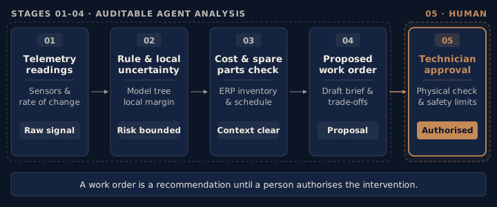 A work order is a recommendation until a person authorises the intervention.
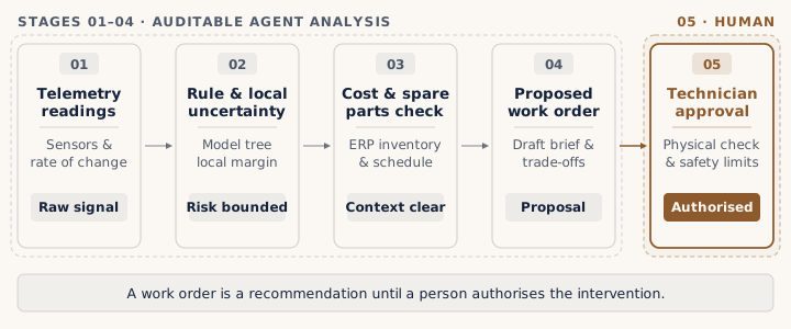 A work order is a recommendation until a person authorises the intervention.
Scroll sideways to explore the full diagram.
Look at what this payload gives the LLM agent:
-
Check the Margin: At 196 minutes of tool wear and 52.4 Nm of torque, the illustrative strain product is 10,270.4, or 729.6 below the example threshold. No rate per hour has been measured, so the agent cannot calculate hours to failure.
-
Counterfactual Operating Adjustment: The agent can compute an operational trade-off:
A 10% reduction in measured torque would give 47.16 Nm and an illustrative strain product of about 9,243.4. A 10% feed-rate change does not guarantee a 10% torque change. A technician must approve any PLC adjustment against machine limits.
-
ERP Spare Parts Check: The agent could ask SAP/Maximo whether a replacement insert is available and draft a maintenance order. A person checks the part and approves any reservation or order.
Instead of treating the score as a dispatch instruction, the agent drafts a work order for review:
“CNC Mill 04 has 196 minutes of tool wear and 52.4 Nm of torque. The illustrative strain product is 10,270.4 against an example threshold of 11,000. Hours to failure are unknown. Please check the sensor readings, part availability and machine limits before approving a work order or changing the PLC.”
The calculation gives the technician something to check. It is not a safety guarantee.
How Did Predictive Maintenance Guide Telecom Dispatch?
In a separate engagement for an unnamed European telecom, we used probabilistic decay modelling to rank line-level failure risk and send crews where risk was highest. The predictive maintenance and capital allocation case study describes that work. It did not use the illustrative CNC model-tree method above.
In telecom infrastructure, reactive dispatch can tie up field crews and leave customers waiting for a fix.
The decision was which lines needed attention before customers were affected.
Basic signal data was not enough. The team added peripheral DSL and hardware telemetry to estimate line-level risk.
The scoring ran on-premise, and the dispatch roster was ranked by predicted failure risk.
The models gave 10–24 hours of warning before failure, giving crews time to plan an intervention.
The engagement recovered £11M a year, a combined effect of network cost savings and revenue retained through reduced churn. That is not a maintenance-only saving or a result of the CNC example.
What Rules Should Govern AI Maintenance Agents?
Give the agent readings and model limits, validate decay estimates, and require human review before dispatch or control changes.
If your engineering team is designing a maintenance or dispatch agent, test it against these three constraints:
- Never pass a raw anomaly score directly to an agent.
An anomaly score is a statistical abstraction. Give the engineer the relevant readings, model limits and reason for the recommendation. - Model continuous decay, not binary death.
A decay estimate can help plan intervention if it is validated against failures and false alarms at the intended decision threshold. - Price the counterfactual before dispatching the crew.
Ask “does slowing the machine down cost less than an unplanned shutdown or a dispatch?” Check the estimate against actual operating limits, parts and a human approval step.
Predictive maintenance can fail when a score has no clear path to an operating decision.
When an agent can show its inputs and limits, the technician can decide whether the risk justifies action.
Do this week
- Ask your engineers what the agent sees. It needs readings and model limits, not a raw anomaly score.
- Ask if the decay estimates are checked against past failures and false alarms.
- Compare the cost of slowing a machine down with an unplanned shutdown or a dispatch.
- Require human approval before any dispatch or control change.
If you are looking to audit your operational AI pipelines, eliminate alarm fatigue, or bridge sensor telemetry to automated field workflows, let’s talk. Review our AI audit advisory or explore how we structured large-scale telecom predictive maintenance.
Frequently asked questions
Why do traditional predictive maintenance alerts cause alarm fatigue?
Static thresholds or anomaly scores can flag benign transient spikes as well as real faults. Repeated false alarms make a warning harder for operators to trust. A useful alert needs context and a decision path.
What is telemetry decay modeling?
A decay model estimates how risk changes over time from telemetry, rather than giving only a yes-or-no fault label. It still needs validation against equipment outcomes before a team uses it to change operations.
How do model trees help an autonomous AI agent schedule maintenance?
A model tree can expose the rule and local coefficients behind a risk estimate. An agent could draft a work order from that estimate, but a technician must check the evidence, parts and safety constraints before approving service or a control change.
What is the commercial ROI of interpretable maintenance models in enterprise operations?
For an unnamed European telecom, probabilistic decay modelling helped rank crews by line-level failure risk and gave 10–24 hours of warning. The engagement recovered £11M a year from combined network cost savings and revenue retained through reduced churn. It did not use the illustrative CNC model-tree method shown here.
Is this where your AI is leaking?
A 45-minute diagnostic shows where the logic between your data and your decisions breaks. No pitch, no deck.
Business
AI in Procurement: Vendor Rationalization with AI Agents
AI in procurement, in practice: how AI agents rationalized a manufacturer's vendors, from requisition to award, while procurement kept the final call.
Business
Who Should Explore AI Tools Inside a Business?
A practical operating rule for assigning AI tool exploration by temperament, not title, so curiosity creates operating memory instead of distraction.
Business
AI Tool Tourism
Why chasing every new AI tool creates cognitive load, workflow breakage, and fragmented productivity — and the three reasons that actually justify a switch.
The Weekly AI Decision Brief